Spiking Performance Evaluation with EWMA

When evaluating the performance of an application it makes sense to run the code several times to get better view on how it performs.

However real world data might be not as perfect as you’d like:

1. Execution times are really bad during your first few executions and then start to get to a somewhat regular state
2. If your tests run on a shared VM then the execution times might spike depending on the workload of the other instances.

The question becomes: Is there a way to remove the noise caused by the initial spike and get a more accurate result than using the noisy average?

A really cool approach is called EWMA which can be used to rate the wireless network quality. It updates the current value with a new one using this formula:

NextValue = OldValue * Alpha + (1 - Alpha) * NewValue

Plotting a series of random data with some spikes and a rough start may look like the blue curve here:

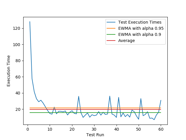
As you can see a high alpha value makes it much more conservative and updates the value more slowly favoring the older values from the beginning. Using a lower value means that newer values are more important and reduces the final value in this case faster.

Here is another example with even harder spikes:

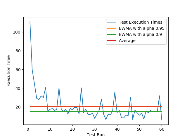
As you can see EWMA with an alpha of 0.9 does a much better job at showing what the real performance values are in this execution environment.

In this last diagram we have a look at how it behaves in case there are no spikes:

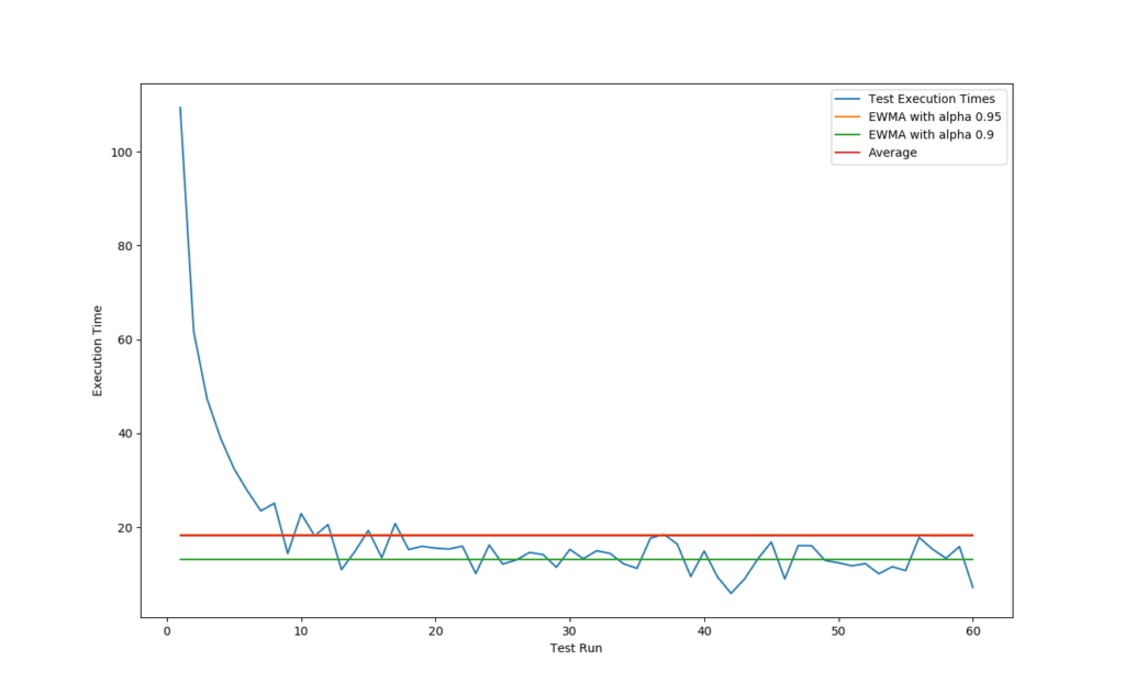
The green line still shows a somewhat accurate representation but probably could use a slight alpha increase to let the low value in the end influence the final value less.

The Script

If you want to play around with the generated values you may use the script below:

import matplotlib.pyplot as plt
import numpy as np
from functools import reduce

# config for sample curve
number_of_tests = 60
worst_duration = 100
perfect_duration = 10
distribution_scale = 3

alpha1 = 0.95
alpha2 = 0.9

def value_generation(x):
    return worst_duration/x + perfect_duration \
           + np.random.normal(0.0, distribution_scale) \
           + np.random.choice([0, 20], p=[0.9, 0.1])

def average(values):
	return sum(values) / len(values)

def ewma(old, new, alpha):
    return old * alpha + (1 - alpha) * new

def ewma01(old, new):
    return ewma(old, new, alpha1)

def ewma02(old, new):
    return ewma(old, new, alpha2)

values = [value_generation(x+1) for x in range(number_of_tests)]
ewma02_val = reduce(ewma02, values)
ewma01_val = reduce(ewma01, values)
average_val = average(values)

plt.figure(1)
t = np.arange(1.0, number_of_tests+1, 1)
plt.xlabel('Test Run')
plt.ylabel('Execution Time')
plt.plot(t, values, '', label='Test Execution Times')
plt.plot(t, [ewma01_val]*60, '', label='EWMA with alpha {}'.format(alpha1))
plt.plot(t, [ewma02_val]*60, '', label='EWMA with alpha {}'.format(alpha2))
plt.plot(t, [average_val]*60, '', label='Average')
plt.legend()

plt.show()